Displaying an image, adding an effect, and optimizing for better performance — by Vuo community member @MartinusMagneson
Transcript
Compositing in Vuo can range from adding a simple filter to creating a large and complex composition that reacts to outside data and generates its own in response. To get into and understand the anatomy of a composition can be a daunting task though, so this tutorial will go through the basics to try and explain the core concepts and workflows to achieve interesting and hopefully good-looking results.
Composition Flow
Composition flow in node-based environments can be split up into two sets. On one hand you’ve got your data; the things you see and use to generate your content. On the other hand, you have the event-flow which decides when stuff happens to your data. Most node-based environments hide the event-flow from the end user to simplify the interaction. This comes at the cost of transparency, efficiency, and flexibility. Vuo exposes this flow to the end user – at the cost of a bit of added complexity. In this part of the tutorial we’ll look at how we can think about event-flow, and how to use it to our advantage to create efficient compositions that might not be viable in other software running on similar hardware.
As this is a compositing tutorial, we will need an input image. For this I will be using Sven Damerow’s “Schachbrett beim aufwärmen” which can be found at Wikimedia Commons.

The number of nodes used in a sketch can vary wildly. Sometimes a seemingly simple task can call for a huge number of nodes, while a seemingly difficult task can be realized using only a couple of nodes.
For this part of the tutorial, I will focus on the former, to explain why you might want to use many nodes to achieve a simple effect – blurring.
Computationally speaking, blurring is a pretty intense task using a convolution matrix. The convolution matrix works by checking the value of every pixel around the active one, and then averages the values of the surrounding pixels. After that it adds the averaged result to the active pixel, usually by a “weight” parameter that decides the amount of influence each pixel should have on the active one. A common matrix is 8 pixels and accounts for all the direct neighbors of the active pixel. However, it can be as low as 1 or take all the pixels in your image into account.
If you have a small image, like 256px X 256px, this means running the matrix calculation 65,536 times. No problem for modern hardware. If your image is a more modern texture size though, a 4,096px X 4,096px image would require about 17 million calculations. That is starting to be somewhat of a task. Especially considering that it must be done at least each 30th of a second. With all our theory done, we can go on to more practical use.
Step 1 – Display an image
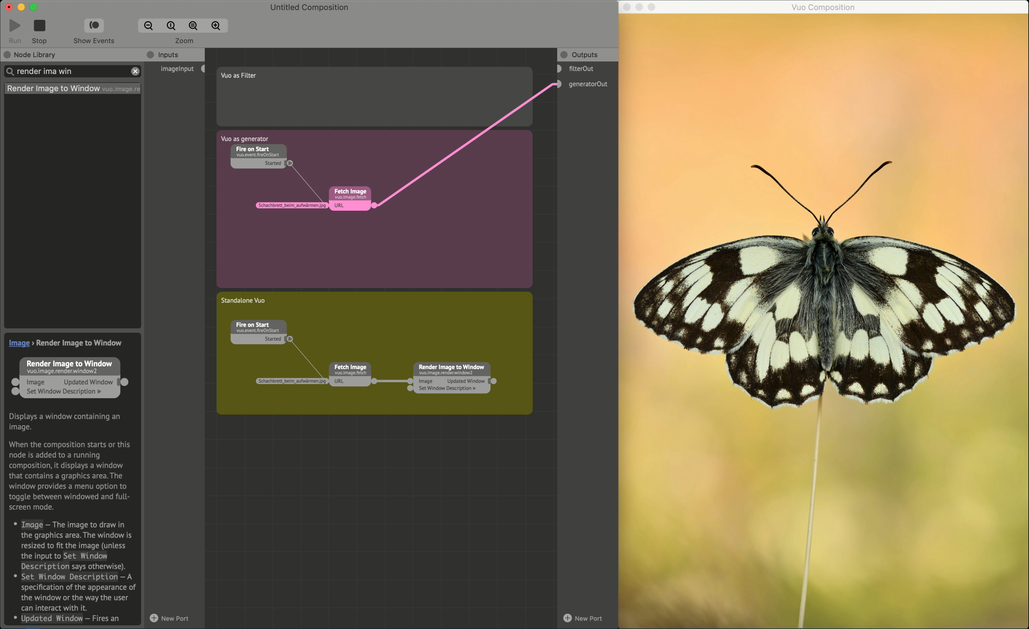
Figure 1 displays the simplest form of image interaction in Vuo three ways. The top, and unpopulated one is Vuo as a filter. Here the image is expected to come from a host application, and thus unpopulated for this example. The middle one is Vuo as a generator inside a host, where the image is produced by Vuo, but output by the host. The bottom one is Vuo as standalone where both the image and output are produced by Vuo.
This example also displays the two main features of Vuo’s control over the data and event flow in the node graph. Thin lines are events, thick lines are data – which also may carry an event signal. The distinction here is important to understand, as it is the control of the event flow that lets you pull off things in Vuo that are hard to do with the same hardware with other solutions. Note that if you’re using a filter protocol the image input will always fire events at the host framerate.
Step 2 – Add an effect
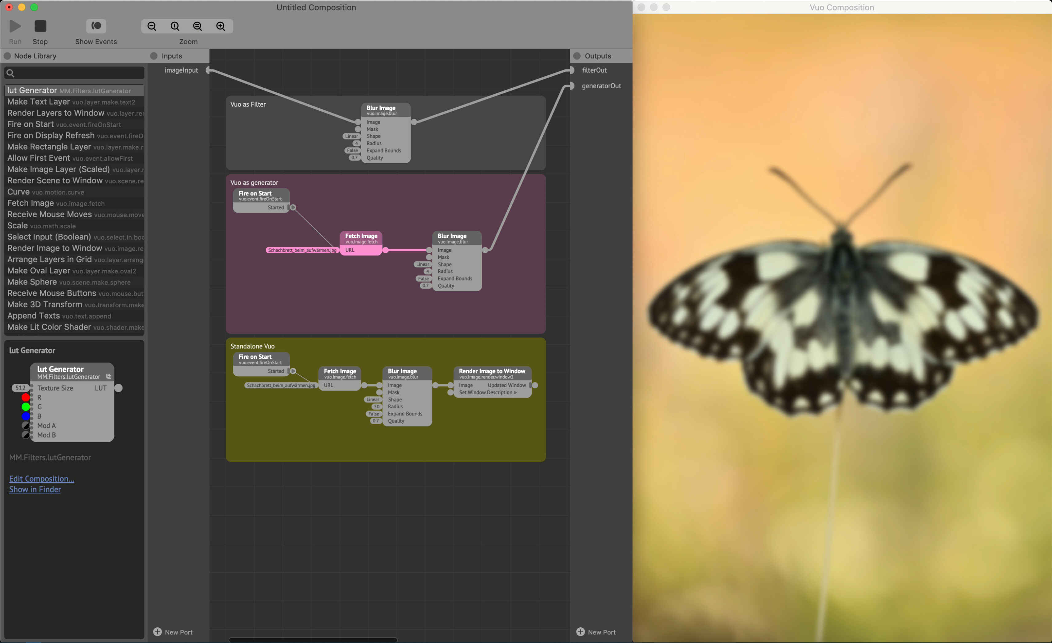
In Figure 2 we blur the image by inserting a blur node between the image input source and the image output. Translated to the flow, we fire an event into the Fetch Image node which adds the image to the sketch. Then we push the image along with the event over to the Blur Image node. This tells the blur node to take the image, process it and then push the blurred image over to the output along with an event. In standalone mode this event tells the Render Image to Window node to render the image to its destination.
Step 3 – Optimize
From here on out, I will only display the standalone mode, but the techniques shown still apply to both the filter and the generator as well.
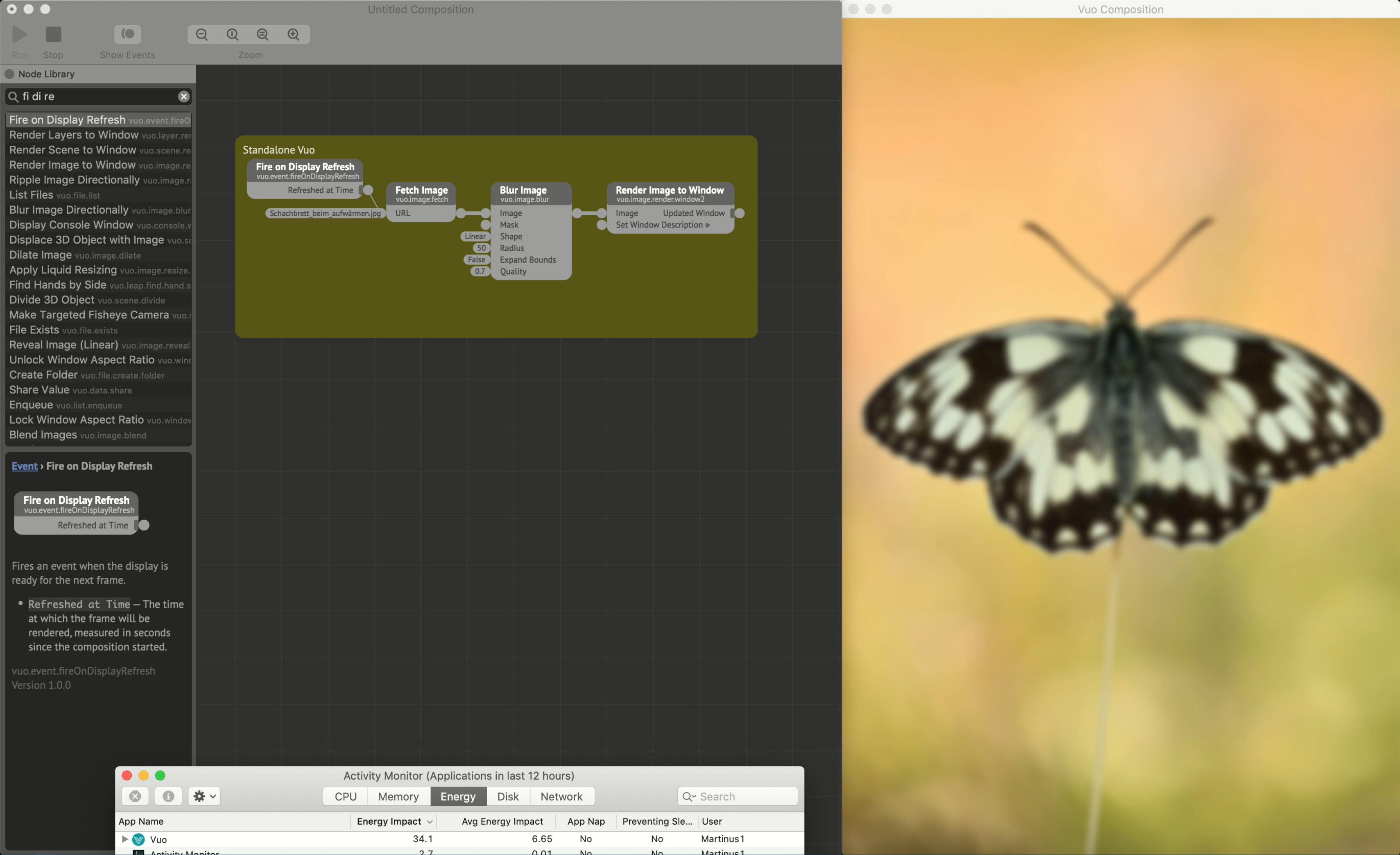
Only having a 2014 Macbook Pro with integrated Intel Graphics, optimization is key to achieve good results on aging and relatively slow hardware. Figure 3 shows the energy impact Vuo has on the computer. It is apparent that it now runs a pretty heavy task that slows it down in general, meaning choppy output and no need for a space heater. Thinking about why there is so much of an energy impact is key to optimizing though.
The first issue is that by using a Fire on Display Refresh node as our event source, we are basically telling Vuo to do the whole operation 60 times a second. The second issue is that we do the operation on an image at its original resolution. This, according to Wikimedia, is 4,852 X 7,278 pixels – or over 35 million pixels. That is trying to process something at near 8K resolution 60 times a second on hardware that barely was made to display 4K (a quarter of the size) video at 30 fps. Luckily, we can do something about both issues!
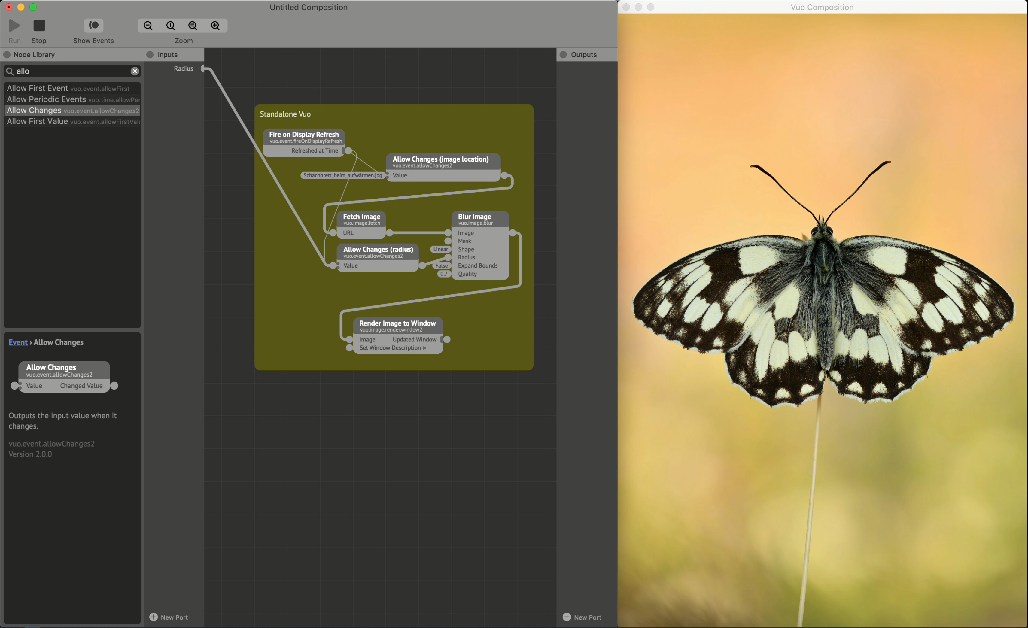
Figure 3.2 shows using the Allow Changes node. This node can be applied to any port type and will only pass through events when the data changes. Event-blocking nodes like this one (Hold Value is another one) are indicated by two dots at the input. These will block any input events until they get a condition to pass them along. You can think of it as a universal gate only allowing for distinctly different items to pass through.
The reason for placing it on the path rather than on the image node itself is that loading an image and comparing it to the previous one is still a relatively high intensity task compared to loading a small string of text and comparing that. Gating the radius (which is the value we want to edit) also ensures that we can have a fader connected to the value and adjust it at a whim, without telling the Blur Image node to process data every frame. Even though this solves our constantly processing issue, the image is still too large for aging and slow hardware, so let’s fix that!
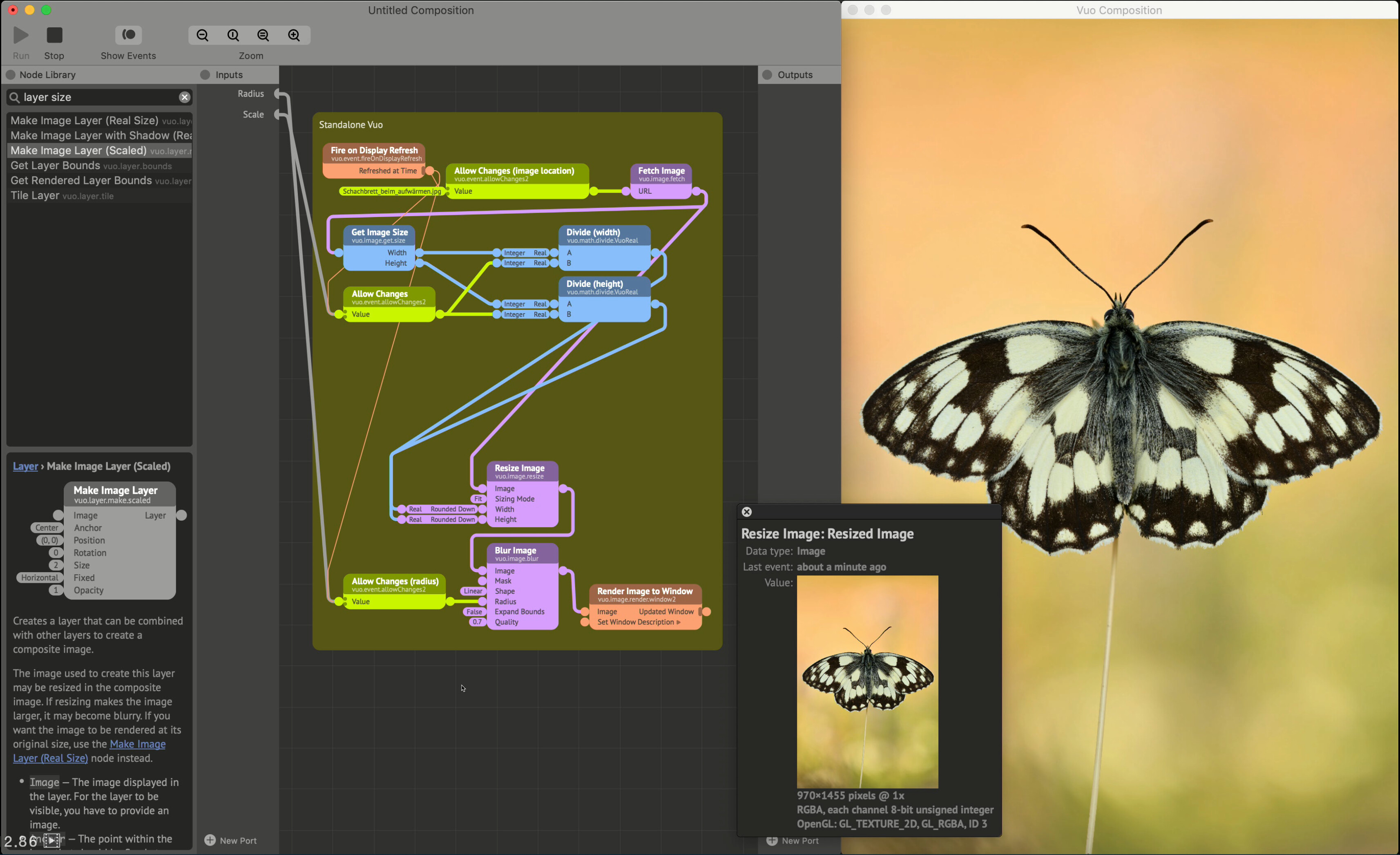
In Figure 3.3 we add a few nodes to resize the image. We get the dimensions of the image when we load it and push the image over to the Resize Image node. If the image doesn’t change, it will be buffered in full in the Resize Image node. Not only is the image buffered, all values on the previous ports are also buffered. This means that when we add two Divide nodes, the only thing changing is the incoming Scale value that we publish – and so, the only event flow we need is from that node to resize the image. Looking at the output port info from the Resize Image node we can see in Figure 3.4 that the image resolution changes.
With the resize in place, we can now smoothly blur the image as shown in Figure 4. Note that the slight stutter/lag comes from the screen recording software, not the actual composition.
 Figure 4Until now, we have only resized the image to a pixel size still larger than what the output window produces. If we were to resize it to a size smaller than this, we would get an unexpected result; the whole window shrinks as shown in Figure 5!
 Figure 5Fortunately, it’s a quick fix. Add another Resize Image node before the final destination, hook it up to your original image dimensions (or the dimensions you want it to render at), and it should stay the same pixel size at the output as at the input (or your desired dimensions). Doing so, the processing happens at a lower resolution, but you get a fixed output result as shown in Figure 6.
Compared to other node-based compositors, this might introduce a few more nodes to scale and display an image, but not an unreasonable amount with the performance improvements in mind. While the event flow control might feel like a hurdle when starting out, the fine-tuning possibilities it gives you are huge – and I’m not aware of similar options in other software.
While blur is a simple effect, and perhaps a bit boring on its own, it is both heavy on hardware, and important for effective compositing. This makes it ideal for an introduction to event flow. For more artistic exploits – read on in part 2 where we’ll take a look at some more advanced techniques for live image manipulation.